
Morphological Classification of Galaxies in S-PLUS using an Ensemble of Convolutional Networks
N. M. Cardoso, G. B. O. Schwarz, L. O. Dias, C. R. Bom, L. Sodre Jr, C. Mendes de Oliveira.
Notas Técnicas do Centro Brasileiro de Pesquisas Físicas, 2021
DOI: 10.7437/NT2236-7640/2021.02.002 Citation
Abstract
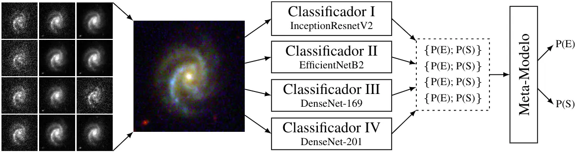
The universe is composed of galaxies that have diverse shapes. Once the structure of a galaxy is determined, it is possible to obtain important information on its formation and evolution. Morphological classification is the cataloging of galaxies according to their visual appearance and it is linked to their physical properties. A morphological classification made through visual analysis is sensible to differences in evaluation among diferent human volunteers. For this reason, systematic, objective and easily reproducible classification of galaxies has been gaining importance since the astronomer Edwin Hubble created his famous classification method. In this work, we combine accurate visual classifications of the Galaxy Zoo project with Deep Learning methods. The goal is to find an efficient technique at human performance level classification, but in a systematic and automatic way, for classification of elliptical and spiral galaxies. For this, a neural network model was created through an Ensemble of four other convolutional models, allowing a greater accuracy in the classification than what would be obtained with any one individual. Details of the individual models and improvements made to these are also described. The present work is entirely based on the analysis of images (not parameter tables) from DR1 (www.datalab.noao.edu) of the Southern Photometric Local Universe Survey (S-PLUS). In terms of classification, we achieved, with the Ensemble, an accuracy of \(\approx 99 \%\) in the test sample (using pre-trained networks).
Online material
Classifications of blind sample
| Column | Description |
|---|---|
| ra | right ascension in decimal degrees (J2000) |
| dec | declination in decimal degrees (J2000) |
| r_auto | S-PLUS DR1 r-band magnitude (SDSS-like r) |
| mn170_pE | probability of the object being elliptical given by the classification of the trained model with objects with magnitude \(r_{auto} < 17\) (mn stands for "MorphoNet") |
| mn170_pS | probability of the object being spiral given by the classification of the trained model with objects with magnitude \(r_{auto} < 17\) |
| mn175_pE | probability of the object being elliptical given by the classification of the trained model with objects with magnitude \(r_{auto} < 17.5\) |
| mn175_pS | probability of the object being spiral given by the classification of the trained model with objects with magnitude \(r_{auto} < 17.5\) |
Downloads:
- Catalog: CSV
- Images: Numpy Arrays
Trained network weights
Weights of trained models as described in the paper. The network was trained with TensorFlow v2 and saved in SavedModel format. Each folder contains the model of a member of the Ensemble. A file in Python3 called MorphoNet Class is available that automates the loading of the weights of each member. It is recommended to use this class instead of making direct predictions as it standardizes member predictions with respect to training data as described in the paper.
Downloads:
- MN170 Weights (1GB): Main • Mirror
- MN175 Weights (1GB): Main • Mirror
- Prediction Class (for both models): MorphoNet Class
Code Samples
import os
import random
import numpy as np
import matplotlib.pyplot as plt
from mpl_toolkits.axes_grid1 import ImageGrid
import morphonet
# kind can be 'mn170' or 'mn175'
mn = morphonet.MorphoNet(kind='mn170', weights_folder='morphonet170')
# this method load the members and meta-model in memory
mn.load()
# load images to memory, using np.load in this case of .npy images
imgs = [np.load(f'colored_splus_stamps_npy/{f}') for f in os.listdir('colored_splus_stamps_npy')]
# call predict method with a list of numpy arrays of shape (128, 128, 3)
preds = mn.predict(imgs)
# select a random sample to plot
ids = random.sample(range(0, len(imgs)), 100)
# plot the reults in a grid
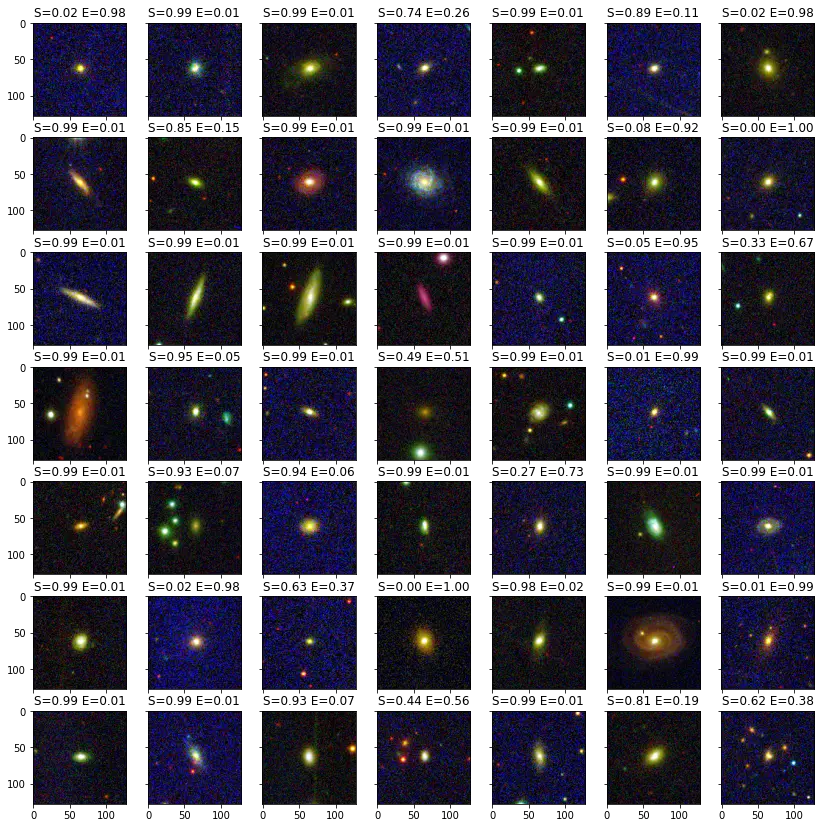
fig = plt.figure(figsize=(14, 16))
grid = ImageGrid(fig, 111, nrows_ncols=(7, 7), axes_pad=0.3)
for ax, _id in zip(grid, ids):
im = imgs[_id]
ax.set_title(f'S={preds[_id][0]:.2f} E={preds[_id][1]:.2f}')
ax.imshow(im)
plt.show()
Citation
@article{cardoso2021,
  title = {Classificação {Morfológica} de {Galáxias} no {S}-{PLUS} por {Combinação} de {Redes} {Convolucionais}},
  volume = {11},
  issn = {22367640},
  url = {https://revistas.cbpf.br/index.php/NT/article/view/140},
  doi = {10.7437/NT2236-7640/2021.02.002},
  number = {2},
  urldate = {2025-01-18},
  journal = {Notas Técnicas},
  author = {Cardoso, N. M. and Schwarz, G. B. and Dias, L. O. and Bom, C. R. and Jr., L. Sodré and De Oliveira, C. Mendes},
  month = oct,
  year = {2021},
  pages = {1--18},
}